A Guide to the Power of `hue` in Seaborn Visualizations

Photo by Robert Katzki on Unsplash

The hue parameter in Seaborn allows for the seamless integration of categorical variables, introducing a spectrum of colors that not only enhances the aesthetic appeal of your plots but also provides a powerful tool for conveying intricate relationships within your data. In this blog, we will embark on a journey to explore the nuances of using ‘hue’ in Seaborn, unlocking its potential to reveal insights, distinguish patterns, and elevate the clarity of your visual narratives.

📊 Usage

Firstly, We will load tips dataset from the online repository in Seaborn. This dataset contains the following data:

One waiter recorded information about each tip he received over a period of a few months working in one restaurant

import seaborn as sns
import matplotlib.pyplot as plt

# Load sample data
data = sns.load_dataset("tips")

Like always, We will inspect our data then:

data.info()

"""
<class 'pandas.core.frame.DataFrame'>
RangeIndex: 244 entries, 0 to 243
Data columns (total 7 columns):
 #   Column      Non-Null Count  Dtype
-- -----     ------------- -----
 0   total_bill  244 non-null    float64
 1   tip         244 non-null    float64
 2   sex         244 non-null    category
 3   smoker      244 non-null    category
 4   day         244 non-null    category
 5   time        244 non-null    category
 6   size        244 non-null    int64
dtypes: category(4), float64(2), int64(1)
memory usage: 7.4 KB
"""

According to the dataset description, each variable has the following meaning:

total_bill: bill in dollars, tip: tip in dollars, sex: sex of the bill payer, smoker: whether there were smokers in the party, day: day of the week, time: time of day, size: size of the party.

Name	Meaning
total_bill	bill in dollars
tip	tip in dollars
sex	sex of the bill payer
smoker	whether there were smokers in the party
day	day of the week
time	time of day
size	size of the party

Scatter Plots

In this example, we’ll compare a simple scatter plot with and without hue to showcase how it can enhance our understanding of the data.

Without hue

sns.scatterplot(x="total_bill", y="tip", data=data)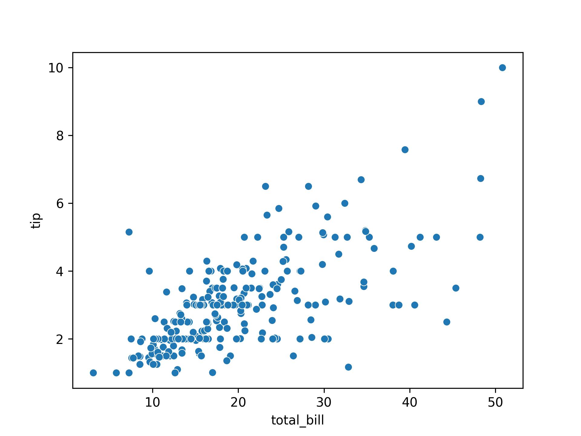

With hue

sns.scatterplot(x="total_bill", y="tip", hue="time", data=data)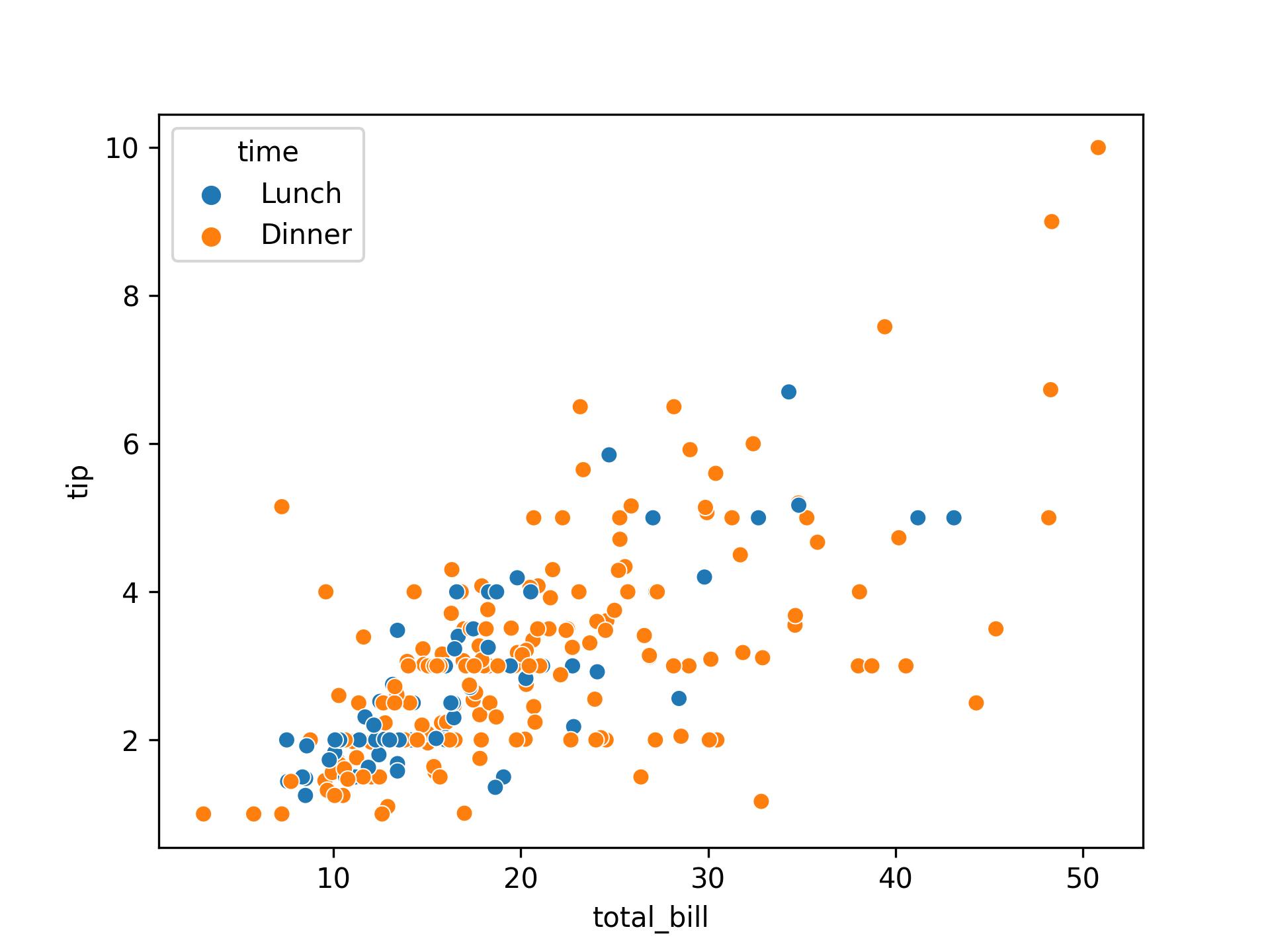

In this example, we compare two scatter plots side by side. The left plot (without hue) shows a basic scatter plot of total bill amount vs. tip without distinguishing different days. The right plot (with hue) introduces the ‘day’ column as the hue parameter, coloring the points based on the days of the week.

By using hue, we can observe how the relationship between total bill and tip varies across different time. This additional categorical information enhances the visualization, making it easier to differentiate patterns and trends within the data.

Bar Plots

sns.barplot(x="day", y="total_bill", hue="sex", data=data)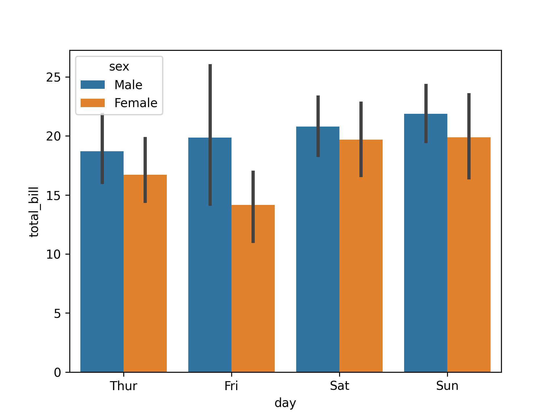

Box Plots

sns.boxplot(x="day", y="total_bill", hue="sex", data=data)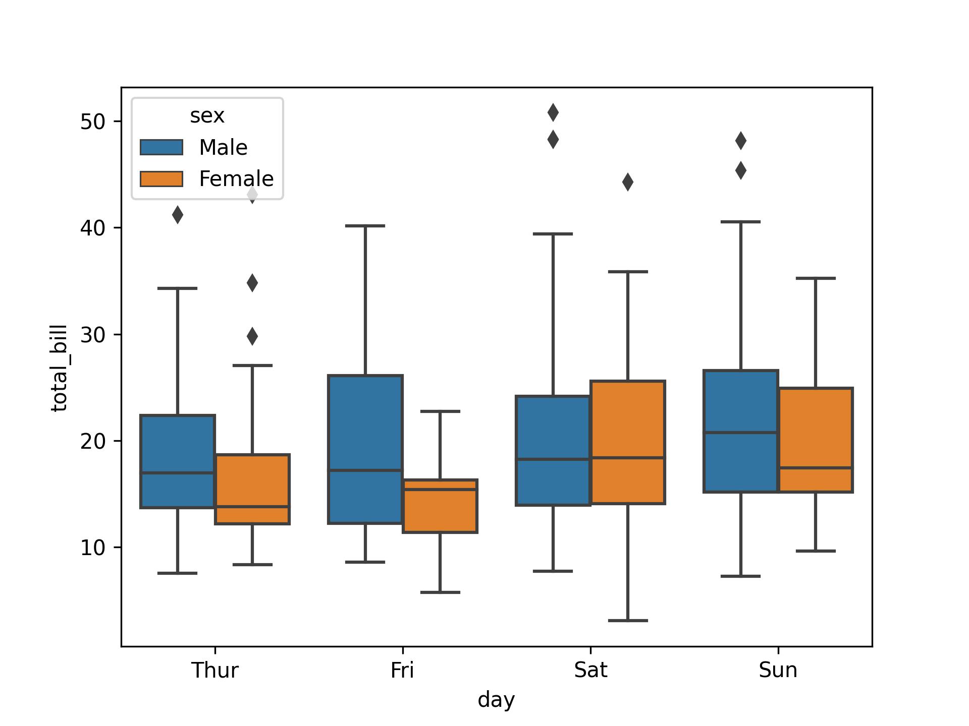

Violin Plots

sns.violinplot(x="day", y="total_bill", hue="sex", data=data)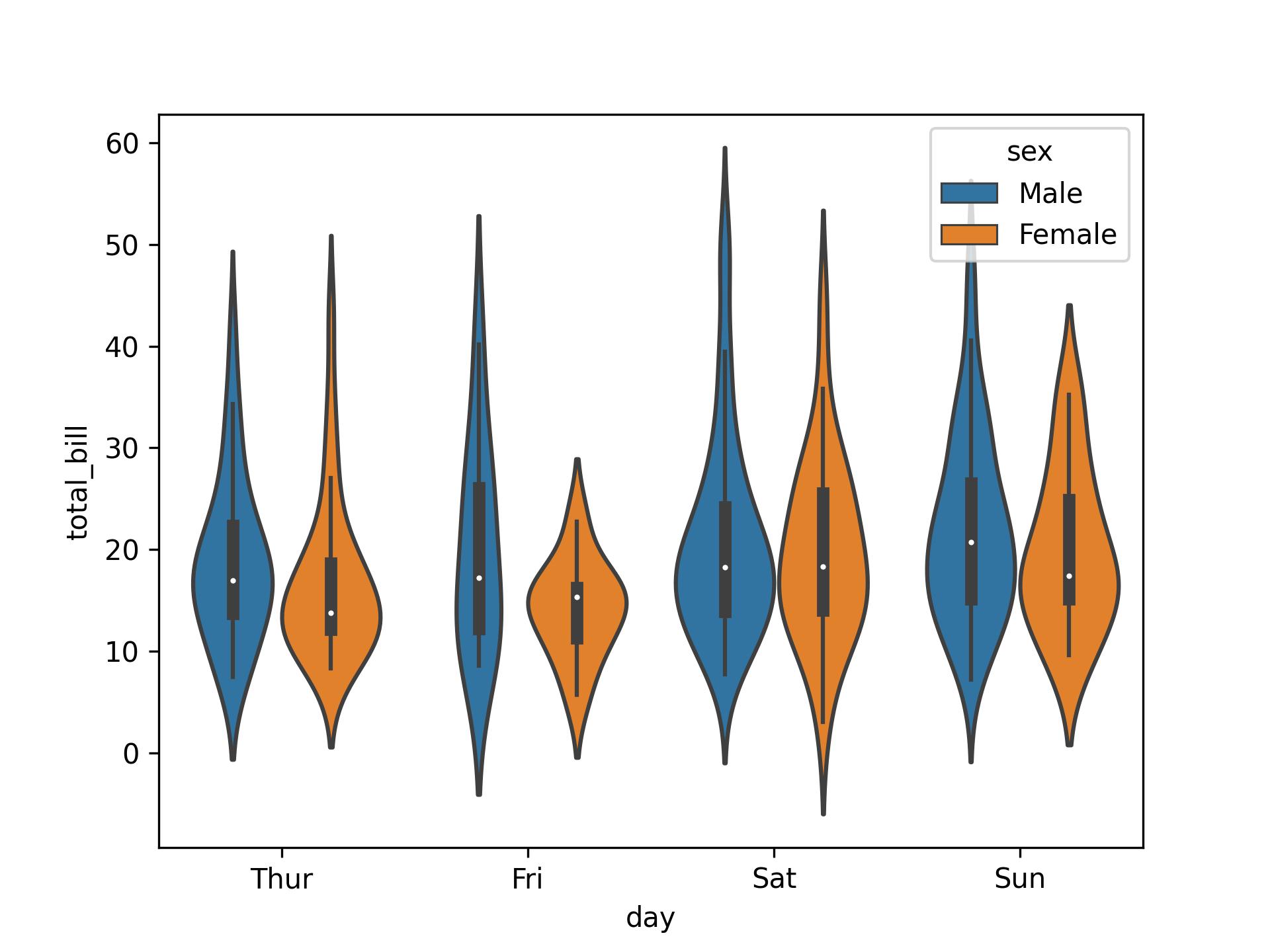

Count Plots

sns.countplot(x="day", hue="sex", data=data)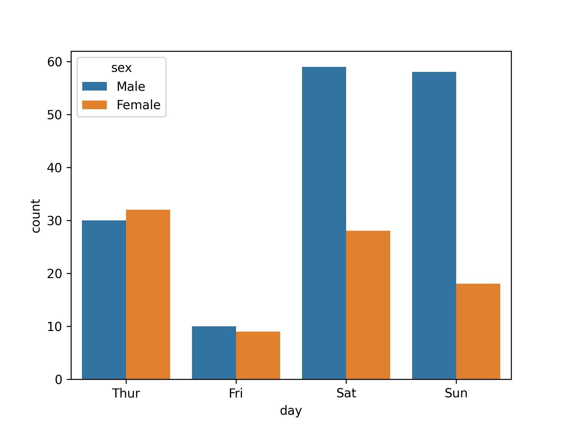

🤔 When to Use and When Not to Use hue?

The use of hue is particularly beneficial in the following cases:

• Visualizing Categorical Relationships: When you are visualizing relationships between two numeric variables and have a third categorical variable that you want to explore simultaneously.

• Highlighting Patterns or Trends: When you want to highlight patterns, trends, or differences in your data by using different colors for different categories.

• Enhancing Interpretability: When you want to enhance the interpretability of your visualizations by adding an extra layer of information through color.

While the hue parameter in Seaborn can be a powerful tool for enhancing visualizations by incorporating an additional categorical variable, there are situations where it might not be necessary or could potentially lead to confusion:

• Limited or No Categorical Data : If your dataset has very limited categorical data or if the categorical variable doesn’t provide meaningful insights into the patterns you are exploring, using hue might not add much value. When the variable specified in hue is not categorical, but rather a continuous variable, using hue may not be appropriate. In such cases, alternative approaches like color gradients or size encoding might be more suitable.

• Overcrowded Plots: When the number of categories within the hue variable is large, it can lead to overcrowded plots with too many colors, making it difficult to distinguish and interpret the information.

• Color Vision Impairments: Consider the audience of your visualizations. If there is a possibility that the audience includes individuals with color vision impairments, relying heavily on color differentiation (such as with hue) might limit accessibility. Ensure your visualizations are still interpretable in grayscale.

Conclusion

In conclusion, Seaborn’s hue parameter is a dynamic tool that breathes vitality into visualizations, providing nuanced insights across plot types, from scatter plots to count plots. By introducing an additional layer of categorical information, hue unveils hidden patterns and relationships. However, its use should be judicious, especially when simplicity is crucial.